Introduction

In the previous post, I introduced you the concepts of NP problem. Travelling Salesman Problem (or TSP) is one of them. I’ll take its definition from Wikipedia:

The travelling salesman problem (TSP) asks the following question: Given a list of cities and the distances 
between each pair of cities, what is the shortest possible route that visits each city exactly once and 
returns to the origin city? It is an NP-hard problem in combinatorial optimization, important in operations 
research and theoretical computer science.

To get a better understanding, take a look at the following picture:

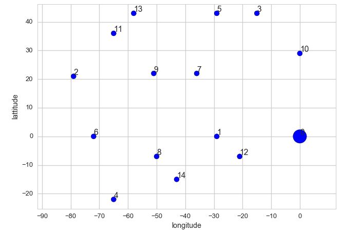
I drawed this map using matplotlib and seaborn with a dataset of locations taken from this page. I will describe the implementation later in this post.

Let’s say each point in the above picture represents a city, so as you can count there are 15 cities in total, from 0 to 14. Now assume that a salesman was given a challenge:

1. Start at any city in the map (says he can teleport at any city at the start of the process)
2. Go to each and every city in the given map to sell a particular mystery product
3. He is allowed to visit each city once only and return to the same city he started
4. The total distance he travelled is the shortest path

In the above figure, there is a point which is bigger than the rest, it represents the city where the salesman started. In our example, we assume he started from city numbered 0, so the point at 0 are drawed with bigger size. (Sorry for the bad representation because the number is so hard to see, I still didn’t find a way to fix that)

Greedy algorithm

One way to solve this problem is to use Greedy algorithm. Basically this algorithm tries to find the best possible solution at each step in the process that satisfy the problem’s requirements. What does it means in this case?

We are trying to find the shortest path for the salesman, so at each step, the best possible solution would be looking for the city which has the closest distance to the last visited city (of course we need to exclude all visited cities except for the last visited one). By repeating this process, we will end up with a shortest path because everytime, we found a city which is closest to the previous visited one.

Start coding

Let’s stop the bullshit theory and get to practice. First, import necessary libraries:

Note: I will use IPython notebook to work with this problem. So please remember that some commands may not 
work if you are using a text editor.

import json
import pandas as pd
import matplotlib as plt
import scipy.spatial.distance as spdist
import numpy as np
import seaborn as sns

%pylab inline
sns.set_context('talk')

Next I will get the dataset. This dataset contains 15 rows, each row is a pair of longitude and lattitude for a city:

# This is the URL for the dataset
url = 'https://people.sc.fsu.edu/~jburkardt/datasets/tsp/p01_xy.txt'

longitudes = []
lattitudes = []

for line in urllib2.urlopen(url):
    # longitude and lattitude are in text, we need to convert them to float, round and convert to integer
    longitude = int(round(float(line.split()[0])))
    lattitude = int(round(float(line.split()[1])))
    
    longitudes.append(longitude)
    lattitudes.append(lattitude)
    
# Build a location pandas Data Frame 
coords = pd.DataFrame({'longitude': longitudes, 'lattitude': lattitudes})

Next, draw the map:

# origin sets the city where the salesman starts his trip
origin = 0

# size of scatter markers, set bigger size for orgin
s = [700 if i == origin else 100 for i in coords.index.values]

# draw 
fig, ax = plt.subplots()
ax.scatter(coords.longitude, coords.lattitude, s=s) 
plt.xticks(xticks)
plt.yticks(yticks)
plt.xlabel('longitude')
plt.ylabel('lattitude')
plt.axis('equal')

# Set annotation for each point
for i in coords.index.values:
    ax.text(coords.longitude[i], coords.lattitude[i], str(i), verticalalignment='bottom')

The result will be the map you already saw at the beginning of this post.

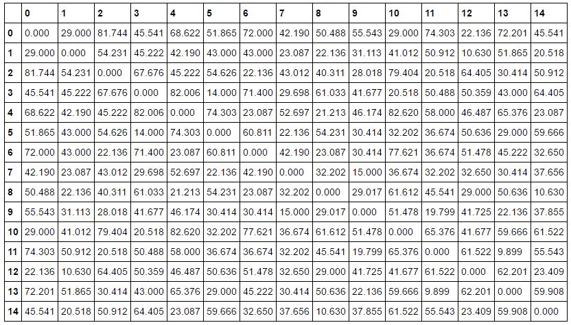
Now, assume that the salesman is in city_0, he needs to look for the city which is closest to city_0 from the remaining 14 candidates. In order to do this easily, I will construct a distance matrix for the input locations. This distance matrix contains the distances (calculated using Euclidean distance) for every city to every other cities.

Scipy has an extremely useful function to help us generating matrices like this. It would be really painful without it.

distance_matrix = pd.DataFrame( ( np.round(spdist.cdist( coords, coords, 'euclidean' ), decimals=3 ) ) )

The cdist() function from Scipy library computes the distance between 2 collections of inputs, so I all I need to do is calculating the distance from the given coordinates with themselves.

Result looks like this, row and column indices are cities:

Now, with this table, I will write a function to find the shortest possible path from the origin to every other cities and back to the starting city itself:

def get_shortest_path(distance_matrix, current_node):
    total_nodes = len(distance_matrix.columns) - 1
    sequence = [current_node]
    t = distance_matrix.T
    t = t.replace(0, np.nan)
    t = t[t.index.values != current_node]

    # Continue until there is no other cities, find the closest cities and add it to the path
    while total_nodes > 0:
        current_node = t[current_node].idxmin()
        sequence.append(current_node)
        
        t = t[t.index.values != current_node]
        total_nodes -= 1
    return sequence

Get the path using above function:

path = get_shortest_path(distance_matrix, origin)
# Append the origin city to the path
path.append(origin)
print path

Output:

[0, 12, 1, 14, 8, 4, 6, 2, 11, 13, 9, 7, 5, 3, 10, 0]

This output shows the most optimal path that our salesman should use to travel from city_0 to all others and back to city_0. Now, let’s change the origin and see if output will change:

origin = 7
path = get_shortest_path(distance_matrix, origin)
# Append the origin city to the path
path.append(origin)
print path

Output:

[7, 9, 11, 13, 5, 3, 10, 0, 12, 1, 14, 8, 4, 6, 2, 7]

The path indeed changed as we observe.

Now let’s draw the map for our salesman:

origin = 0
path = get_shortest_path(distance_matrix, origin)
path.append(origin)
s = [700 if i == origin else 100 for i in coords.index.values]

# draw 
fig, ax = plt.subplots()
ax.scatter(coords.longitude, coords.lattitude, s=s) 
plt.xticks(xticks)
plt.yticks(yticks)
plt.xlabel('longitude')
plt.ylabel('lattitude')
plt.axis('equal')

# Set annotation for each point
for i in coords.index.values:
    ax.text(coords.longitude[i], coords.lattitude[i], str(i), verticalalignment='bottom')
    
i = 0
while i < len(path) - 1:
    first = path[i]
    second = path[i+1]
    coord_x = list(coords.loc[[first, second], 'longitude'])
    coord_y = list(coords.loc[[first, second], 'lattitude'])
    i += 1
    plt.plot(coord_x, coord_y, 'r')   

Note that I had to redraw the points because otherwise it just displays that path, without points. Let’s take a look at the output:

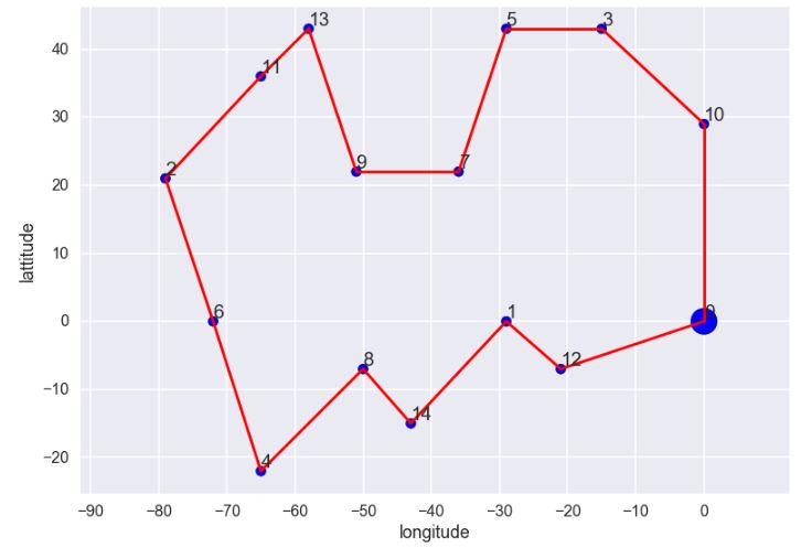
Nice! Let’s see the output with different origin = 7:

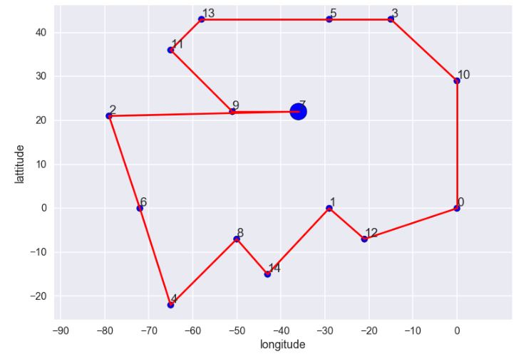
Note that because cities city_2, city_9 and city_7 are almost straight so it looks like the salesman has to go from city_7 back to city_9 twice, but in fact he’s not.

Conclusion

In both solutions, we observe both requirements are satisfied:

• The salesman must go to each and every city once only
• The distance that he travels is the shortest. We know this because at each step, we chose the city which is closest to the previous one.

You can try to change the origin to see different output.